2) Add More Than One New Row or Column
As you play around with your data, you might find you're
constantly needing to add more rows and columns. Sometimes, you may even
need to add hundreds of rows. Doing this one-by-one would be super tedious. Luckily, there's always an easier way.
To add multiple rows or columns in a spreadsheet, highlight the same
number of preexisting rows or columns that you want to add. Then,
right-click and select "Insert."
In the example below, I want to add an additional three rows. By
highlighting three rows and then clicking insert, I'm able to add an
additional three blank rows into my spreadsheet quickly and easily.
3) Filters
When you're looking at very large data sets, you don't usually need
to be looking at every single row at the same time. Sometimes, you only
want to look at data that fit into certain criteria. That's where
filters come in.
Filters allow you to pare down your data to only look at certain rows
at one time. In Excel, a filter can be added to each column in your
data -- and from there, you can then choose which cells you want to view
at once.
Let's take a look at the example below. Add a filter by clicking
the Data tab and selecting "Filter." Clicking the arrow next to the
column headers and you'll be able to choose whether you want your data
to be organizing in ascending or descending order, as well as which
specific rows you want to show.
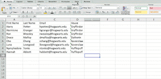
In my Harry Potter example, let's say I only want to see the students
in Gryffindor. By selecting the Gryffindor filter, the other rows
disappear.
4) Remove Duplicates
Larger data sets tend to have duplicate content. You may have a list
of multiple contacts in a company and only want to see the number of
companies you have. In situations like this, removing the duplicates
comes in quite handy.
To remove your duplicates, highlight the row or column that you want
to remove duplicates of. Then, go to the Data tab, and select "Remove
Duplicates" (under Tools). A pop-up will appear to confirm which data
you want to work with. Select "Remove Duplicates," and you're good to
go.You
can also use this feature to remove an entire row based on a duplicate
column value. So if you have three rows with Harry Potter's information
and you only need to see one, then you can select the whole dataset and
then remove duplicates based on email. Your resulting list will have
only unique names without any duplicates.
5) Transpose
When you have low rows of data in your spreadsheet, you might decide
you actually want to transform the items in one of those rows into
columns (or vice versa). It would take a lot of time to copy and paste
each individual header -- but what the transpose feature allows you to
do is simply move your row data into columns, or the other way around.
Start by highlighting the column that you want to transpose into
rows. Right-click it, and then select "Copy." Next, select the cells on
your spreadsheet where you want your first row or column to begin.
Right-click on the cell, and then select "Paste Special." A module will
appear -- at the bottom, you'll see an option to transpose. Check that
box and select OK. Your column will now be transferred to a row or vise
versa.
6) Text to Columns
What if you want to split out information that's in one cell into two
different cells? For example, maybe you want to pull out someone's
company name through their email address. Or perhaps you want to
separate someone's full name into a first and last name for your email
marketing templates.
Thanks to Excel, both are possible. First, highlight the column that
you want to split up. Next, go to the Data tab and select "Text to
Columns." A module will appear with additional information.
First, you need to select either "Delimited" or "Fixed Width."
- "Delimited" means you want to break up the column based on characters such as commas, spaces, or tabs.
- "Fixed Width" means you want to select the exact location on all the columns that you want the split to occur.
In the example case below, let's select "Delimited" so we can separate the full name into first name and last name.
Then, it's time to choose the Delimiters. This could be a tab,
semi-colon, comma, space, or something else. ("Something else" could be
the "@" sign used in an email address, for example.) In our example,
let's choose the space. Excel will then show you a preview of what your
new columns will look like.
When you're happy with the preview, press "Next." This page will
allow you to select Advanced Formats if you choose to. When you're done,
click "Finish."
Excel Formulas
7) Simple Calculations
In addition to doing pretty complex calculations, Excel can help you
do simple arithmetic like adding, subtracting, multiplying, or dividing
any of your data.
- To add, use the + sign.
- To subtract, use the - sign.
- To multiply, use the * sign.
- To divide, use the / sign.
You can also use parenthesis to ensure certain calculations are done
first. In the example below (10+10*10), the second and third 10 were
multipled together before adding the additional 10. However, if we made
it (10+10)*10, the first and second 10 would be added together first.Bonus: If you want the average of a set of numbers, you can use the formula =AVERAGE(Cell Range). If you want to sum up a column of numbers, you can use the formula =SUM(Cell Range).
8) Conditional Formatting Formula
Conditional formatting allows you to change a cell's color based on
the information within the cell. For example, if you want to flag
certain numbers that are above average or in the top 10% of the data in
your spreadsheet, you can do that. If you want to color code
commonalities between different rows in Excel, you can do that. This
will help you quickly see information the is important to you.
To get started, highlight the group of cells you want to use
conditional formatting on. Then, choose "Conditional Formatting" from
the Home menu and select your logic from the dropdown. (You can also
create your own rule if you want something different.) A window will pop
up that prompts you to provide more information about your formatting
rule. Select "OK" when you're done, and you should see your results
automatically appear.
9) IF Statement
Sometimes, we don't want to count the number of times a value
appears. Instead, we want to input different information into a cell if
there is a corresponding cell with that information.
For example, in the situation below, I want to award ten points to
everyone who belongs in the Gryffindor house. Instead of manually typing
in 10's next to each Gryffindor student's name, I can use the IF
THEN Excel formula to say that if the student is in Gryffindor, then they should get ten points.
The formula: IF(logical_test, value_if_true, value of false)
Example Shown Below: =IF(D2="Gryffindor","10","0")
In general terms, the formula would be IF(Logical Test, value of true, value of false). Let's dig into each of these variables.
- Logical_Test: The logical test is the "IF" part of the statement. In this case, the logic is D2="Gryffindor"
because we want to make sure that the cell corresponding with the
student says "Gryffindor." Make sure to put Gryffindor in quotation
marks here.
- Value_if_True: This is what we want the cell to show if the value is true. In
this case, we want the cell to show "10" to indicate that the student
was awarded the 10 points. Only use quotation marks if you want the
result to be text instead of a number.
- Value_if_False: This is what we want the cell to show if the value is false. In this case, for any student not in Gryffindor, we want the cell to show "0" to show 0 points. Only use quotation marks if you want the result to be text instead of a number.
10) Dollar Signs
Have you ever seen a dollar sign in an Excel formula? When used in a
formula, it isn't representing an American dollar; instead, it makes
sure that the exact column and row are held the same even if you copy
the same formula in adjacent rows.
You see, a cell reference -- when you refer to cell A5 from cell C5,
for example -- is relative by default. In that case, you're actually
referring to a cell that's five columns to the left (C minus A) and in
the same row (5). This is called a relative formula. When you copy a
relative formula from one cell to another, it'll adjust the values in
the formula based on where it's moved. But sometimes, we want those
values to stay the same no matter whether they're moved around or not --
and we can do that by making the formula in the cell into what's called
an absolute formula.
To change the relative formula (=A5+C5) into an absolute formula,
we'd precede the row and column values by dollar signs, like this:
(=$A$5+$C$5). (Learn more on Microsoft Office's support page here.)
Source:http://blog.hubspot.com/marketing/how-to-use-excel-tips#sm.00008itjql7kod95td01v8rgf583h


0 comments:
Post a Comment